Tokenization

This is the most important step: converting text into numbers. This decision effects how model handles code, math, emojis, and rare words.

Neural network models do not understand text as we do. They only know how to work with numbers. Therefore, if we want to build neural network based language models (LLMs), we need a way to convert text into numbers. This process is called “tokenization.”

We use different tokenizers to achieve this. In this article, we will discuss two modern tokenizers, the BPE tokenizer and the Unigram tokenizer. Almost every LLM that we see uses one of these.

Note that many people also mention SentencePiece, but SentencePiece is not a tokenizer of its own. It uses either BPE or Unigram underneath. We will discuss more about it in the SentencePiece section.

So how do we convert text into numbers?

We know that a computer doesn't understand text, right? Like, it only understands bits (0, 1). So how did we help the computer understand language?

From ASCII to Unicode

The first step was ASCII (American Standard Code for Information Interchange). ASCII uses 7 bits to represent a symbol/character/number. So that's 2^7 = 128 possibilities.

('A' -> 65 -> 1000001)
('B' -> 66 -> 1000010)
('C' -> 67 -> 1000011)

So when we want to encode HELLO using ASCII, it becomes:

72 69 76 76 79

which eventually becomes:

01001000 01000101 01001100 01001100 01001111

The initial bit is zero in all cases because ASCII only uses 7 bits to represent a character.

ASCII only has 128 characters. It can represent English well, but how about representing emojis and other languages?

So Unicode was born.

In Unicode, every character gets a unique number:

(A -> U+0041)
(B -> U+0042)
(中 -> U+4E2D)
(😀 -> U+1F600)

This number is often called a Unicode code point.

The Unicode code point is written in hexadecimal format. We then need a way to convert this hexadecimal code point into raw bytes.

We use UTF encodings to convert these Unicode code points into raw bytes. There are various types of UTF encodings, out of which UTF-8 is the most commonly used.

So there is a Unicode code point for different characters in different languages, and we can then use encodings to convert these code points into raw bytes. Each byte contains 8 bits (0s and 1s), which can finally be understood by the computer.

This is how computers understand text in different languages and different symbols.

So, we already have a way to convert text into numbers. We can use the same representation that computers use to process text. So why do we need all these tokenizers? We could directly convert text into byte values and pass them to neural network based language models.

The reason is that we want these models to understand semantic relationships. For example, the model should understand that the words “dog” and “cat” belong to a similar category. To learn such semantic relationships, models need high dimensional vector representations.

So, do we have an embedding vector for every word such as “dog”, “cat”, and every other word in the language? That would be difficult because there are a huge number of words in the English language. Furthermore, we want our models to be able to process out of vocabulary words, which are words that are not present in the model’s dictionary.

For example, suppose the model’s dictionary contains embedding vectors for the subwords “un”, “happy”, and “ness”, but does not contain an embedding vector for the word “unhappiness”. The model can still process the word because it can be broken down into these smaller subwords.

So we may have characters, subwords, and words in the model’s vocabulary. You might ask that it is enough to have characters in the vocabulary because everything can be broken down into characters. So, if we have an embedding vector for every character (English), (a-z), and (A-Z), we can process all the text, but this is computationally inefficient.

Because the word “dog” now gets broken down into 3 characters, and each character has its respective embedding. But in modern neural network based language models, we use the attention mechanism, and it is the crux of the language model, where every token attends to every other token. As the number of tokens increases, the amount of computation required also increases. Moreover, the model has to learn the meaning of words from sequences of character tokens rather than receiving meaningful subwords or words directly. This makes learning semantic relationships more difficult. So we make the model’s job easier by looking for commonly occurring subwords and words and providing them with separate embedding vectors.

We use the words “dog” and “cat” very often, so we provide embedding vectors for them. Now the model can more easily learn semantic relationships. But how do we decide which subwords and words get separate embedding vectors? This is decided by tokenizers.

Byte Pair Encoding (BPE)

This tokenizer starts with the 256 ID's in it's vocabulary i.e byte values (0-255). So each byte value from 0-255 is already in the tokenizer's vocabulary.

Following the idea from this original BPE Gage's BPE paper paper, we repeatedly replace the most frequently occurring byte pairs with a new token ID, starting from 256, because a byte value can never be greater than 255.

So, how do we build it? We first have a dataset that is used to train the tokenizer. In our vocabulary, we already have 256 IDs (0–255), corresponding to all possible byte values. We then increase the vocabulary size by replacing the most commonly occurring byte pairs with new IDs starting from 256. This process is repeated until the desired vocabulary size is reached.

First of all, the text in the dataset is converted into bytes (UTF-8). For example, the character 'e' is replaced with the number 101. So we get a list of integers from the input text. All the integers in this list will be less than or equal to 255 (≤ 255). That's because a byte can represent a maximum value of 255.

Now, all we need to do is find the most commonly occurring pairs. Let's say that, out of the given list of integers, the pair (101, 102) occurs most frequently. We then replace all occurrences of the pair (101, 102) with a new ID, and these new IDs start from 256.

So now, we replace all (101, 102) pairs with 256. This ID, 256, represents two letters ("ef") — [101 → 'e', 102 → 'f'].

After replacing all occurrences of (101, 102) with 256, we search for the next most commonly occurring pair and replace that pair with 257. This process continues until we reach the target vocabulary size.

While training the tokenizer, we keep a note of the byte pairs that we are replacing and the new IDs we are assigning to them. So, by the end of the tokenizer training process, we have a dictionary:

{
    (101,102): 256,
    (196,250): 257,
    ...
    (256,257): 9836,
    ...
}

Encode and Decode

So, we now have a tokenizer. But how do we use this tokenizer to convert text into numbers and numbers back into text?

For that, we use two functions: Encode and Decode.

The Encode function first converts the input text into bytes; let's call them input bytes. The Encode function then checks whether there is any pair in the input bytes that exists in the dictionary obtained during tokenizer training. If such a pair exists, it replaces that pair with the corresponding ID.

We keep replacing all pairs in the input bytes that are present in the dictionary until there are no more replaceable pairs left.

Let's say our input bytes are:

[200,198,65,79,101,102,196,250,68,93]

There is a pair (101,102), so we replace it with 256. Now we also have a pair (196,250), so we replace that pair with 257.

At this point, the input bytes become:

[200,198,65,79,256,257,68,93]

Do we stop here? No.

Look carefully: the pair (256,257) is also present in the dictionary. So we replace that pair with the ID 9836.

The input bytes now become:

[200,198,65,79,9836,68,93]

In this way, we keep replacing byte pairs until there is no pair left in the input bytes that exists in the dictionary.

So, this is how we convert text into token IDs. The Encode function converts text into token IDs.

But how can we convert these token IDs back into text?

For that, we use the Decode function, which converts token IDs back into text.

From Bytes to Subwords

Note that, under the hood, we are actually merging frequently occurring byte pairs, but from a higher-level perspective, we are effectively merging frequently occurring subwords or words.

Let's understand this better.

In the GPT-2 tokenizer (the tokenizer used by GPT-2, which has a vocabulary size of 50,257), there is a token ID 5347 corresponding to " ing". This means that, under the hood, we were merging the bytes corresponding to the characters 'i', 'n', and 'g'. However, when viewed from a larger lens, what we are really doing is merging a frequently occurring subword unit.

So while BPE technically operates on byte pairs, the repeated merging process eventually creates meaningful subword tokens such as " ing", "tion", "ingly", and even entire words that occur frequently in the training data.

BPE tokenizer is all about repeatedly merging the most frequent pairs.

This algorithm is popularized for LLMs by the GPT2 paper - Language Models are Unsupervised Multitask Learners

However, this paper mentions an issue with the BPE algorithm. There are many instances of the same word appearing with different punctuation marks, such as "dog.", "dog!", etc. This wastes vocabulary because the same word appears in multiple variations. To avoid this, the text is first split using a set of rules that essentially separate punctuation, numbers, and characters. BPE is then applied independently to each part, which helps solve this issue.

Even in the case of BPE in general, we usually split the text at whitespace boundaries and apply BPE independently to each word. This is because, if we apply BPE directly to raw text, it may create tokens that cross word boundaries and enter another word, such as "ing and". We do not want this to happen. Additionally, different languages often require language-specific rules for splitting text before applying BPE independently to each segment.

SentencePiece

Modern LLMs often use SentencePiece, an efficient library for training tokenizers. It supports both BPE and Unigram tokenization algorithms. We will study the Unigram tokenizer in a later section. First, however, let us understand the problem that SentencePiece is trying to solve, as introduced in the paper - SentencePiece: A simple and language independent subword tokenizer

SentencePiece removes this preprocessing step before applying subword tokenization algorithms and instead applies these algorithms directly to raw text. The original GitHub repository describes SentencePiece as:

"SentencePiece implements subword units (e.g., byte-pair encoding (BPE) and unigram language models) with the extension of direct training from raw sentences. SentencePiece allows us to build a purely end-to-end system that does not depend on language-specific pre/post-processing."

How did they achieve this? The main idea is surprisingly simple. SentencePiece replaces the space character with a special symbol, ▁, and treats it as a normal character. This allows the tokenizer to preserve word boundary information while operating directly on raw text. As a result, there is no need for language-specific preprocessing tools before training the tokenizer.

The GitHub repository also mentions that SentencePiece supports the Unigram Language Model in addition to BPE. So, let's understand what a Unigram tokenizer is.

The Unigram Tokenizer

The Unigram model is fundamentally different from BPE. In contrast to BPE, which starts with a small vocabulary and repeatedly merges frequent token pairs, the Unigram model starts with a very large vocabulary. This initial vocabulary is generally a superset containing all characters in the corpus, many substrings up to a certain length, and often some BPE-generated pieces as well. The algorithm then repeatedly removes tokens from this vocabulary until the desired vocabulary size is reached.

Let me try to explain how Unigram tokenization works.

First, we have a text corpus. From this corpus, we construct an initial vocabulary. As mentioned earlier, this vocabulary is typically a superset containing all characters in the corpus, many substrings up to a certain maximum length, and some additional BPE-style pieces. Let us assume that our text corpus contains the following words:

hug
hugs
pug
pun
bun

From this, let us assume that the Unigram model constructs the following initial vocabulary:

h
u
g
p
b
n
s

hu
ug
pu
un
bu

hug
hugs
pug
pun
bun

Now, we calculate an initial probability for each token in the vocabulary, roughly based on frequency heuristics.

After this step, every token in the vocabulary is assigned a probability.

Next, we generate all possible segmentations of each word and score each segmentation using the token probabilities we have obtained.

Let us assume that we have the following token probabilities:

P(ug)=0.107
P(hug)=0.071
P(hugs)=0.036
P(h)=0.071
P(g)=0.107
P(u)=0.178
P(s)=0.036
P(hu)=0.071

We generate all possible segmentations of every word and score them using the token probabilities. Let us consider the word "hug":

[hug] : P([hug])=0.071
[h] [ug] : P([h][ug])=P([h])P([ug])= 0.071 * 0.107= 0.0076
[hu] [g] : P([hu][g])=P([hu])P([g])= 0.071 * 0.107= 0.0076
[h] [u] [g] : P([h][u][g])= 0.071 * 0.178 * 0.107= 0.00135
Total : 0.08755
Now Let's normalize these probabilities:
[hug] -> 0.811
[h] [ug] -> 0.087
[hu] [g] -> 0.087
[h] [u] [g] -> 0.015
Now these are probabilities of a segmentations of certain words P (S | word)

Now let's also generate all the possible segmentations of the word "hugs":

[hugs] : P([hugs])=0.036
[hug] [s] : P([hug][s])=P([hug])P([s])=0.071 * 0.036 = 0.002556
[h] [ug] [s] : P([h][ug][s])=P([h])P([ug])P([s])=0.071*0.107*0.036 = 0.000273
We can also generate more segmentations but for the sake of simplicity let's limit these now and normalize them so we will have probabilities of segementations of word 'hugs'

Similarly, we can do this for the other words in the corpus.

The EM Algorithm: E-step and M-step

Now, we calculate the expected count of each token in the vocabulary.

To compute these expected counts, we use the following formula. This step is called the E-step (Expectation Step):

Formally, define freq(t) as the expected count of token t summed over all possible

Let us calculate freq(hug).

To calculate this, we need to look at all possible segmentations of all the words in the corpus and check whether the token "hug" appears in a given segmentation. If it does, we take the probability of that segmentation and add it to the total. By summing these probabilities across all segmentations of all words, we obtain the expected count (or frequency) of the token.

Let us do this:

Word: hug

[hug]           (contains hug)         -> P([hug])         = 0.811
[h] [ug]        (does not contain hug) -> 0
[hu] [g]        (does not contain hug) -> 0
[h] [u] [g]     (does not contain hug) -> 0

Word: hugs

[hugs]          (does not contain hug) -> 0
[hug] [s]       (contains hug)         -> P([hug][s])     = 0.065
[h] [ug] [s]    (does not contain hug) -> 0
[h] [u] [g] [s] (does not contain hug) -> 0

Therefore,

freq(hug) = 0.811 + 0.065 = 0.876

We perform the same calculation for every token in the initial vocabulary. Once we have the expected counts of all tokens, we update their probabilities using:

P(token) = frea(token)

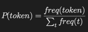
The probabilities obtained from this step become the updated token probabilities. This step is called the M-step (Maximization Step).

Notice that we obtained:

freq(hug) = 0.876

This value is called the expected count of the token. In reality, the token "hug" may appear only once in the corpus, but after averaging over all possible segmentations weighted by their probabilities, its expected count becomes 0.876.

We then use these newly updated probabilities and repeat the same process again:

E-step -> Compute expected counts
M-step -> Update token probabilities

This process continues until the probabilities converge. Convergence means that the token probabilities stop changing significantly between successive iterations. For example:

Iteration 1:
P(hug) = 0.120

Iteration 2:
P(hug) = 0.156

Iteration 3:
P(hug) = 0.161

Iteration 4:
P(hug) = 0.162

Iteration 5:
P(hug) = 0.162

Since the probabilities are no longer changing appreciably, we say that the EM algorithm has converged.

Pruning the Vocabulary

The actual process now works as follows.

First, we calculate the likelihood of the corpus.

After EM convergence, we obtain the probabilities of all tokens in the vocabulary. Using these probabilities, we calculate the probability of every possible segmentation of each word and sum them together. We call this value P(word).

The likelihood of the corpus is then calculated as:

-log (word)

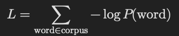
Now, we remove a token from the vocabulary and calculate the likelihood of the corpus again. We repeat this process for every token in the vocabulary and compute an importance score for each token:

score(t) = Lwithout & - Lwith t

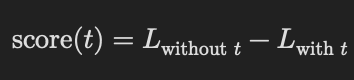
A smaller score means that removing the token does not significantly affect the corpus likelihood, indicating that the token is less important and can be removed from the vocabulary.

For example, if our initial vocabulary contains 100,000 tokens, we would need to perform this computation for every token, which is extremely expensive in practice.

The exact computation would look something like this:

for piece in current_vocab:
    ll = current_loss  # computed using all segmentations of all words

    remove(piece)

    run_EM_until_convergence()

    ll2 = loss_without_piece

    delta[piece] = ll2 - ll

remove_piece_with_smallest_delta()

However, rerunning EM for every token is computationally infeasible.

To avoid this, SentencePiece approximates the value of delta(piece) instead of computing it exactly.

The approximation used by SentencePiece is roughly as follows:

for piece in current_vocab:

    # Find the second-best segmentation of the piece itself
    alternative = second_best_segmentation(piece)

    # Run Viterbi on the entire corpus
    # (only the best segmentation of each word is used)
    viterbi_paths = Viterbi(corpus)

    # Count token frequencies from the Viterbi paths
    freq(token) = count of token in viterbi_paths

    # Compute current unigram probabilities
    P(token) = freq(token) / sum(freq)

    # Pretend that the piece is removed
    # and replaced by its second-best segmentation

    for each occurrence of piece:
        replace piece with alternative

    # Update frequencies and total token count
    new_freq(token)
    new_sum

    # Compute new probabilities after replacement
    P'(token) = new_freq(token) / new_sum

    F = freq(piece) / sum(freq)

    delta[piece] = F * (log(P(piece)- Σ log(P'(alternative_token))))

rank pieces by delta

keep pieces with the largest delta

remove pieces with the smallest delta

Tokens whose removal causes only a small decrease in likelihood are considered unimportant and are removed. Tokens whose removal causes a large decrease in likelihood are considered important and are retained in the vocabulary.

SentencePiece not only optimizes this particular aspect, but its implementation is also written in C++, which makes it extremely fast.